
Understanding Optimizers in ML Model Training
Published:
An optimizer in the context of machine learning is a crucial component responsible for adjusting the parameters of a model during the training process to minimize the error or loss function.
Essentially, an optimizer determines how the model learns by iteratively updating the model parameters based on the gradients of the loss function with respect to those parameters. Optimizers play a vital role in training machine learning models efficiently and effectively. They enable models to learn from data by finding the optimal set of parameters that minimize the discrepancy between the predicted outputs and the ground truth labels. Without optimizers, the process of training a machine learning model would be impractical, as manually adjusting the parameters to minimize the loss function would be extremely laborious and time-consuming. Thus, optimizers automate and streamline the training process, allowing machine learning models to learn and improve their performance over time, ultimately leading to better predictive accuracy and generalization to unseen data.
A summary graph can be found below to help understand the evolution of the multiple optimizers introduced in this blog.
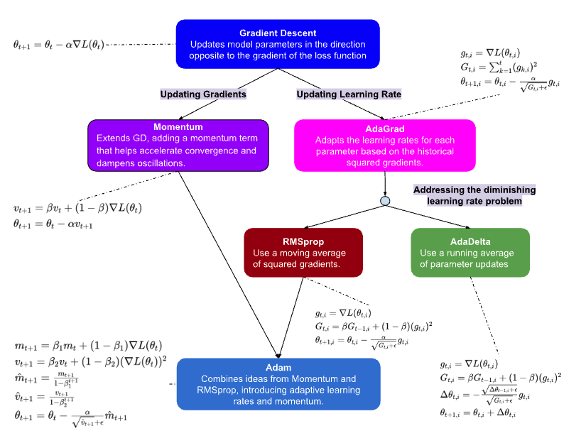
Optimizers
Following shows the equations representing the update rules for the parameters $\theta$ in each iteration of the optimization process for the respective algorithms.
Gradient Descent
Gradient Descent is one of the simplest yet fundamental optimization algorithms used in machine learning and deep learning. Its core principle involves iteratively updating model parameters in the direction opposite to the gradient of the loss function with respect to those parameters. By taking steps proportional to the negative of the gradient, Gradient Descent aims to minimize the loss function and thereby improve the model’s performance.
\[\begin{equation*} \begin{aligned} \theta_{t+1} & = \theta_{t} - \alpha \nabla L(\theta_{t}) \end{aligned} \end{equation*}\]Where:
- $\theta_t$ is the parameter vector at time step $t$.
- $\alpha$ is the learning rate.
- $L(\theta_t)$ is the loss function.
Momentum
Momentum is an optimization algorithm that addresses some of the limitations of Gradient Descent, particularly its slow convergence in certain cases. By introducing the concept of momentum, this algorithm accelerates the convergence by accumulating a velocity vector that keeps track of the past gradients’ directions. By incorporating momentum, the updates to the parameters not only depend on the current gradient but also on the accumulated past gradients, resulting in smoother and faster convergence.
\[\begin{equation*} \begin{aligned} v_{t+1} & = \beta v_{t} + (1 - \beta) \nabla L(\theta_{t}) \\ \theta_{t+1} & = \theta_{t} - \alpha v_{t+1} \end{aligned} \end{equation*}\]Where:
- $v_t$ is the velocity at time step $t$.
- $\beta$ is the momentum parameter.
AdaGrad
AdaGrad, Adaptive Gradient Algorithm, is an adaptive learning rate optimization algorithm that adjusts the learning rates for each parameter based on the historical gradients’ magnitudes. Unlike traditional optimization methods with fixed learning rates, AdaGrad individually scales the learning rates for each parameter, allowing more aggressive updates for infrequent parameters and smaller updates for frequent ones. This adaptivity enables AdaGrad to effectively handle sparse and noisy data, making it suitable for a wide range of optimization problems.
\[\begin{equation*} \begin{aligned} g_{t,i} & = \nabla L(\theta_{t,i}) \\ G_{t,i} & = \sum_{k=1}^{t} (g_{k,i})^2 \\ \theta_{t+1,i} & = \theta_{t,i} - \frac{\alpha}{\sqrt{G_{t,ii} + \epsilon}} g_{t,i} \end{aligned} \end{equation*}\]Where:
- $g_{t,i}$ is the gradient of the parameter $i$ at time step $t$.
- $G_{t,i}$ is the accumulated squared gradients.
- $\epsilon$ is a small constant to prevent division by zero.
AdaDelta
AdaDelta, Adaptive Delta, is a variant of AdaGrad that seeks to address its drawback of monotonically decreasing learning rates, which can eventually lead to overly aggressive updates and premature convergence. By replacing the learning rate with a dynamically adjusted parameter that accumulates past gradients’ squares, AdaDelta effectively adapts the learning rate without requiring an initial learning rate specification. This self-adaptivity makes AdaDelta particularly robust to noisy gradients and suitable for training deep neural networks.
\[\begin{equation*} \begin{aligned} g_{t,i} & = \nabla L(\theta_{t,i}) \\ G_{t,i} & = \beta G_{t-1,ii} + (1 - \beta) (g_{t,i})^2 \\ \Delta\theta_{t,i} & = - \frac{\sqrt{\Delta\theta_{t-1,i} + \epsilon}}{\sqrt{G_{t,i} + \epsilon}} g_{t,i} \\ \theta_{t+1,i} & = \theta_{t,i} + \Delta\theta_{t,i} \end{aligned} \end{equation*}\]Where:
- $\Delta\theta_{t,i}$ is the parameter update at time step $t$.
- $\beta$ is the decay rate for the moving average.
- $\epsilon$ is a small constant to prevent division by zero.
RMSprop
RMSprop, Root Mean Square Propagation, is another adaptive learning rate optimization algorithm designed to mitigate AdaGrad’s diminishing learning rates issue. By introducing a decay factor that exponentially averages past squared gradients, RMSprop adjusts the learning rates based on the recent gradient magnitudes, leading to more stable and effective updates. This adaptive behavior allows RMSprop to converge faster and more reliably, especially in scenarios with sparse or non-stationary gradients.
\[\begin{equation*} \begin{aligned} g_{t,i} & = \nabla L(\theta_{t,i}) \\ G_{t,i} & = \beta G_{t-1,i} + (1 - \beta) (g_{t,i})^2 \\ \theta_{t+1,i} & = \theta_{t,i} - \frac{\alpha}{\sqrt{G_{t,i} + \epsilon}} g_{t,i} \end{aligned} \end{equation*}\]Adam
Adam, Adaptive Moment Estimation, is a popular optimization algorithm that combines the advantages of both momentum and RMSprop. By maintaining exponentially decaying averages of past gradients and squared gradients, Adam adapts the learning rates for each parameter while also incorporating momentum-like behavior.
This adjustment in learning rates is achieved through the adaptive moment estimation of the first and second moments of the gradients ($m_t$ and $v_t$ respectively), which are used to scale the parameter updates. While there isn’t a distinct learning rate associated with each parameter, the adaptive nature of Adam allows it to effectively adjust the magnitude of updates based on the historical behavior of gradients, akin to having parameter-dependent learning rates.
This adaptive moment estimation enables Adam to converge quickly and efficiently, often outperforming other optimization algorithms in various deep learning tasks.
\[\begin{equation*} \begin{aligned} m_t & = \beta_1 m_{t-1} + (1 - \beta_1) g_t \\ v_t & = \beta_2 v_{t-1} + (1 - \beta_2) (g_t)^2 \\ \hat{m}_t & = \frac{m_t}{1 - \beta_1^t} \\ \hat{v}_t & = \frac{v_t}{1 - \beta_2^t} \\ \theta_{t+1} & = \theta_t - \frac{\alpha}{\sqrt{\hat{v}_t} + \epsilon} \hat{m}_t \end{aligned} \end{equation*}\]AdamW
AdamW, Adam with Weight Decay, is an extension of the Adam optimizer that introduces weight decay regularization directly into the optimization process. By incorporating weight decay, which penalizes large parameter values, AdamW helps prevent overfitting and improves generalization performance. This modification enhances the stability and robustness of Adam, making it particularly well-suited for training deep neural networks with large-scale datasets.
\[\begin{equation*} \begin{aligned} \theta_{t+1} & = \theta_t - \frac{\alpha}{\sqrt{\hat{v}_t} + \epsilon} (\hat{m}_t + \lambda \theta_t) \end{aligned} \end{equation*}\]Where:
- $\lambda$ is the weight decay parameter.