This blog is part of the “Deep Learning in Depth” series, where I’ll dive into the world of PyTorch. It aims to provide fundamental concepts and advanced techniques of PyTorch through coding examples.

Tensors

Tensors serve as the fundamental data components in PyTorch.

PyTorch tensors are multidimensional arrays optimized for numerical computations, capable of storing numeric data types such as float32, int32, and more. They adopt a contiguous memory layout similar to arrays in C/C++, enabling efficient data access and vectorized operations. This layout proves advantageous, particularly when leveraging hardware acceleration like SIMD (Single Instruction, Multiple Data) instructions on CPUs or CUDA on Nvidia GPUs.

In comparison to objects like Python lists, tensors offer several advantages in deep learning computations:

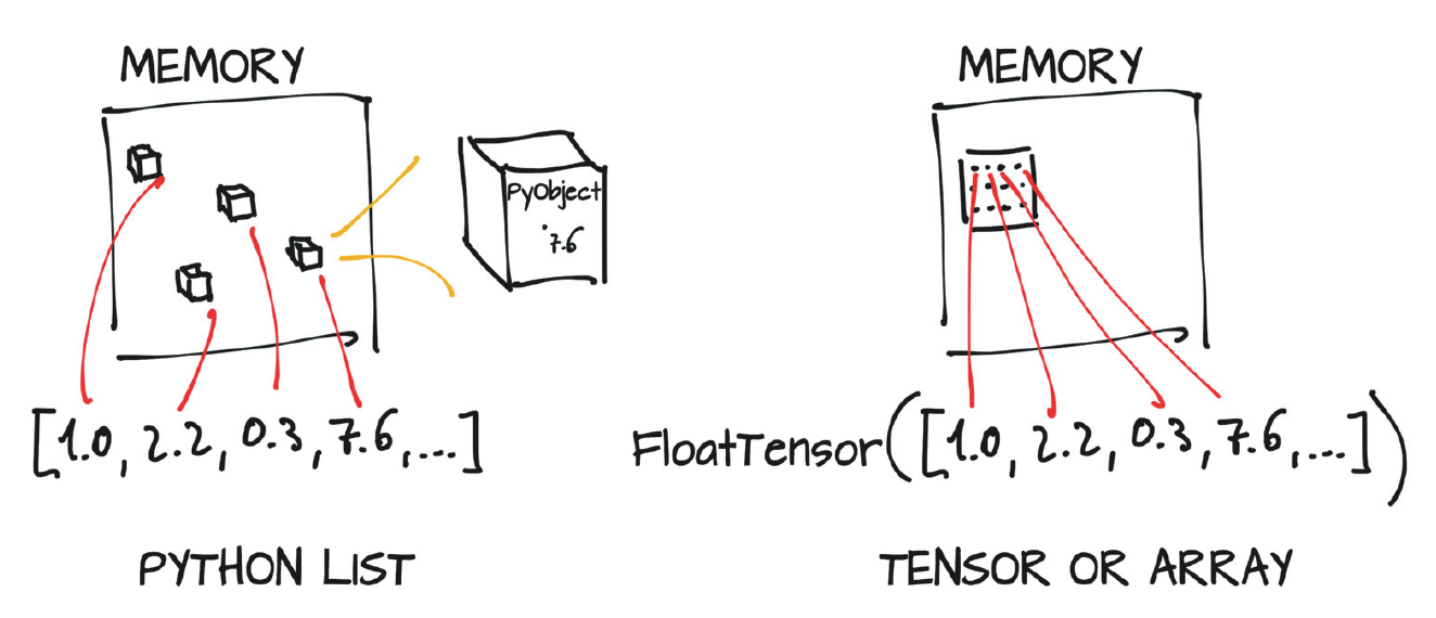
• Python lists internally manage an array of pointers to objects of any data type. These objects are not stored in a contiguous memory block. Consequently, when the list undergoes resizing due to appending beyond its current capacity, it necessitates the allocation of a new array and the copying of elements from the old array, potentially incurring memory reallocation overhead.

• Python treats numbers as full-fledged objects, entailing additional memory overhead due to object encapsulation, reference counting, and other Python-specific features.

Figure 1 shows the differences in memory allocation for PyTorch tensors and Python lists (Book: Deep Learning with PyTorch).

• Figure 1: Python object numeric values (boxed) and PyTorch tensor numeric*
• values (unboxed array)* #{figure-1}

Data Types

PyTorch defines a long list of tensor types with the data types mentioned in the tensors webpage.

I’ll use torch.float32, torch.float16 and torch.bfloat16 as examples to understand how the choice of data types can affect the ML modeling.

Float32

As mentioned in wikipedia, the IEEE 754 standard specifies a Float32 in binary with 32 bits of:

• Sign bit: 1 bit
• Exponent width: 8 bits
• Significand precision: 24 bits (23 explicitly stored)

The example digits are shown in Figure 2.

Figure 2: The bits of a 32 bits float number. {#figure-2}

The real value assumed by a given 32-bit data with a given sign, biased exponent e, and a 23-bit fraction:

The ranges of the components are:

• $\text{sign}$ is either 0 or 1.
• $E \in {1, \ldots, 254 }$,
• $1.b_{22}b_{21}…b_{0} \in {1, 1+2^{-23}, \ldots, 2-2^{-23}}$

Therefore the range of the float32 number is $[-3.4e^{+38}, \, 3.4e^{+38}]$.

Float16 and BFloat16

The data type of float16 has exponent width of 5 bits and 10 significand precision bit, while bfloat16 has 8 and 7 respectively.

Both Float16 and BFloat16 have half of the digits compared to Float32. The Float16 data type can express values in the range $\pm65,504$, with the minimum value above 1 being $1 + 2^{-10}$. BFloat16 sacrifices the precision, but it preserves the exponent bits maintaining the Float32’s range. the minimum value above 1 being $1 + 2^{-7}$.

In deep learning, BFloat16 has the advantage over Float16:

• Exponent Range: BFloat16’s larger exponent range (same as float32) reduces overflow/underflow issues.
• Numerical Stability: More stable training dynamics due to wider range.
• Ease of Use: Simplified transition from float32, reducing mantissa without exponent changes.
• Hardware Support: Optimized implementations in modern AI hardware.
• Efficiency: Similar memory and computational benefits as float16 with better stability.

These factors collectively make bfloat16 a favorable choice over float16 for many deep learning applications, particularly when dealing with large models and datasets where numerical stability and hardware efficiency are critical.

It is worth noting that the 16-bit floating-point, half-precision data type is notably absent from standard CPUs. However, it holds prominence within modern GPUs, primarily due to its advantageous characteristics in specific high-performance computing tasks. This adoption is largely fueled by the demands of applications such as machine learning, where the pronounced benefits of FP16, particularly in terms of speed and efficiency, are highly consequential.

Other Data Types and Tensor Creation

PyTorch provides various data types for integers, including int64, int32, and int16. By default, an integer tensor is created with a data type of int64 unless otherwise specified.

For example,

double_points = torch.ones(10, 2) # -> torch.int64
normal_points = torch.zeros(10, 2, dtype=torch.int) # -> torch.int32
short_points = torch.tensor([[1, 2], [3, 4]], dtype=torch.short) # -> torch.int16
cast_double_points = short_points.double() # -> torch.int64

Storage

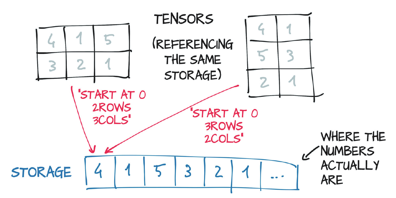
A storage is a one-dimensional array of numerical data, such as a contiguous block of memory containing numbers of a given type. However, tensors can be viewed in different dimensionality. It is emphasized in Figure 3.

Figure 3: Tensors are views over a Storage instance. Storages are 1-dimentional, while the tensors can be viewed in higher dimentions. {#figure-3}

Size, Offset, and Strides

In the context of tensors, understanding the concepts of size, storage offset, and strides is crucial for effective manipulation and optimization.

Size (Shape in NumPy)

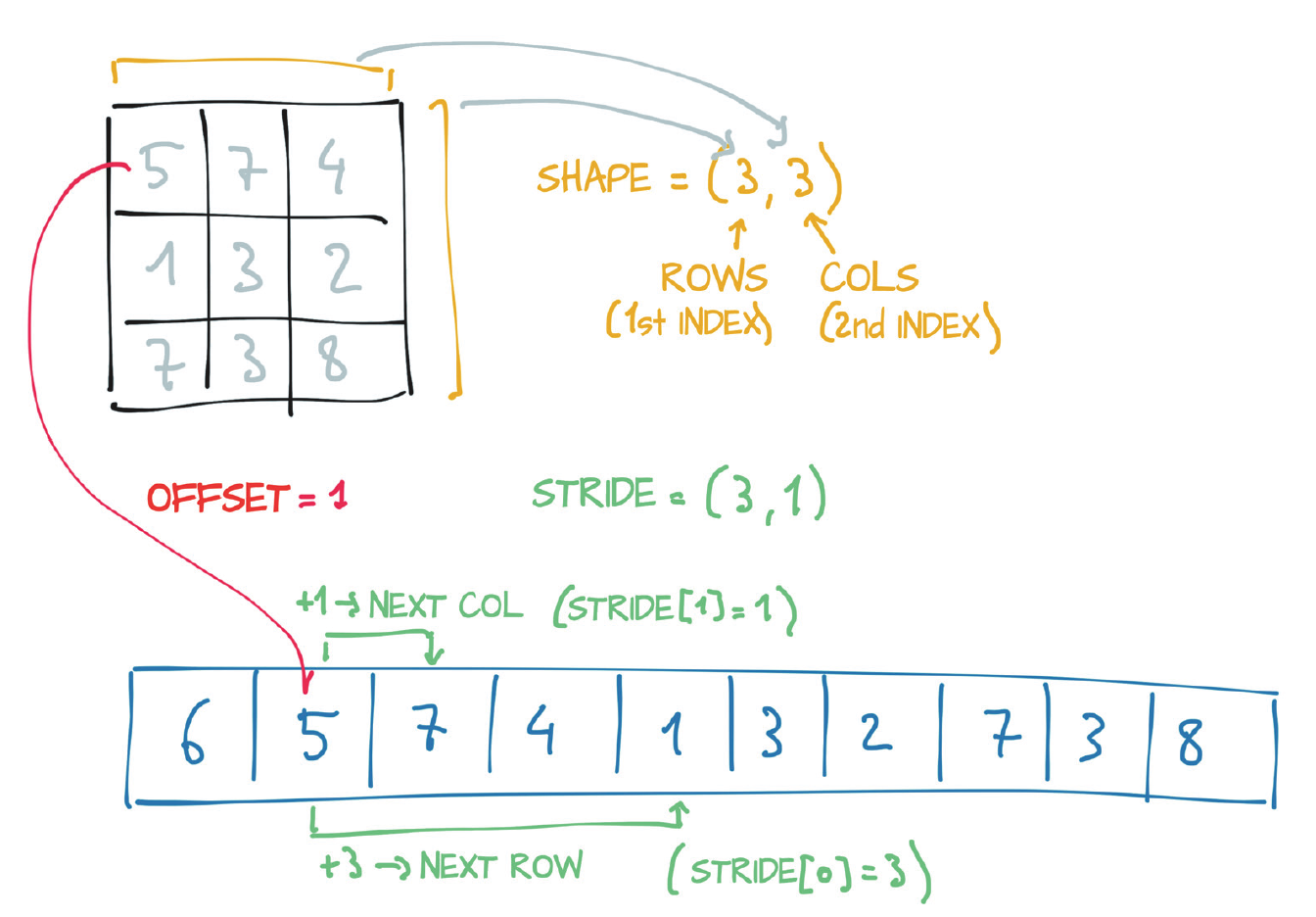
The size, or shape in NumPy terminology, is a tuple that specifies the number of elements along each dimension of the tensor. For example, a tensor with a size of (3, 4) has 3 rows and 4 columns.

Offset

The storage offset is the position in the underlying storage array where the first element of the tensor is located. This offset allows the tensor to reference its data correctly within a larger storage array.

Stride

The stride is a tuple that indicates the number of elements to skip in the storage array to move to the next element along each dimension of the tensor. For instance, a stride of (4, 1) means moving 4 elements in the storage array to go to the next row and 1 element to move to the next column.

These concepts are visualized in Figure 4.

Figure 4: Relationship among a tensor’s offset, size, and stride. {#figure-4}

Contiguity in Memory

The relationship between Tensors and Storage facilitates efficient operations, such as transposing a tensor or extracting a subtensor. These operations are computationally inexpensive because they do not involve memory reallocation. Instead, they create a new tensor object with adjusted size, storage offset, or stride values, maintaining the same underlying data.

The storage array holds the elements of the tensor sequentially, row by row. As a result, a transposed tensor becomes non-contiguous in memory. To rearrange the elements and make the tensor contiguous again, you can use the contiguous() function. Here’s an example of such a scenario.

points = torch.tensor([[1.0, 4.0], [2.0, 1.0], [3.0, 5.0]])
points.storage() # -> [1.0, 4.0, 2.0, 1.0, 3.0, 5.0]
points_t = points.t() # -> [[1.0, 2.0, 3.0], [4.0, 1.0, 5.0]]
points.is_contiguous() # -> True
points_t.is_contiguous() # -> False
points_t_cont = points_t.contiguous() # update the storage.
points_t_cont.is_contiguous() # -> True
points_t_cont.storage() # -> [1.0, 2.0, 3.0, 4.0, 1.0, 5.0]

Moving to GPU

PyTorch enables the seamless transfer of tensors to GPU(s), facilitating massively parallel, high-speed computations. Tensors can be directly created on GPUs or transferred from the CPU using the to() function. Examples are provided below:

points_gpu = torch.tensor([[4.0, 1.0], [5.0, 3.0]], device='cuda')
points_gpu = points_cpu.to(device='cuda') # same as: device='cuda:0'
points_gpu = points_cpu.cuda() # OR: points_cpu.cuda(0)

These methods enable efficient utilization of GPU resources, enhancing the performance of computations, particularly in scenarios requiring intensive parallel processing.

NumPy Interoperability

PyTorch tensors can be efficiently converted to NumPy arrays using the Tensor.numpy() method, and vice versa (torch.from_numpy()), thanks to zero-copy interoperability facilitated by the shared storage system that works with the Python buffer protocol.

The returned NumPy array shares the same underlying buffer as the tensor storage. Consequently, the conversion to a NumPy array incurs virtually no overhead, provided the data is in CPU RAM. Any modifications made to the NumPy array will directly affect the originating tensor.

Serialization

PyTorch uses pickle to serialize tensor objects, along with dedicated serialization code for the storage.

with open('../data/p1ch3/ourpoints.t', 'wb') as f:
    torch.save(points, f)

with open('../data/p1ch3/ourpoints.t', 'rb') as f:
    points = torch.load(f)

This approach allows for quick tensor saving and loading within PyTorch, but the resulting file format is not interoperable with other software.

For projects that require interoperable tensor storage, the HDF5 format and library is a suitable alternative. HDF5 is a portable, widely supported format for representing serialized multidimensional arrays, organized in a nested key-value structure. Python supports HDF5 through the h5py library, which handles data in the form of NumPy arrays.

Autograd

PyTorch’s autograd system provides automatic differentiation, allowing gradients to be computed automatically during the backward pass of neural network training. This simplifies the implementation of gradient-based optimization algorithms such as backpropagation.

The tensors can track their origin, remembering the operations and parent tensors from which they were derived. Given any forward expression, regardless of its complexity, PyTorch can automatically provide the gradient of that expression with respect to its input parameters.

To enable PyTorch to automatically calculate gradients during backpropagation, the parameters must have requires_grad=True:

params = torch.tensor([1.0, 0.0], requires_grad=True)
# Model computation and loss calculation
loss = loss_fn(model(t_u, *params), t_c)
loss.backward()  # Compute gradients

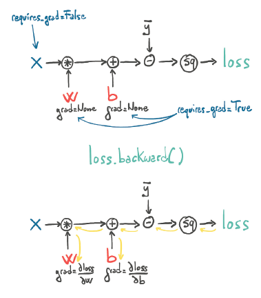
When the backward() function is called, PyTorch will calculate the gradients of the loss with respect to the parameters. This process is crucial for optimizing model parameters during model training.

The forward and backward computation graphs generated by autograd during model training are illustrated in Figure 5.

Figure 5: The forward and backward graphs of the model as computed by autograd. {#figure-5}

Gradient Accumulation

Gradients in PyTorch are accumulated by default, which means each call to backward() adds the new gradients to any existing gradients stored in the tensor’s .grad attribute. Without resetting the gradients, they accumulate across multiple backward passes, leading to incorrect updates.

Zeroing out gradients ensures that each optimization step only considers the gradients from the current forward and backward pass, leading to correct and isolated weight updates.

Optimizers

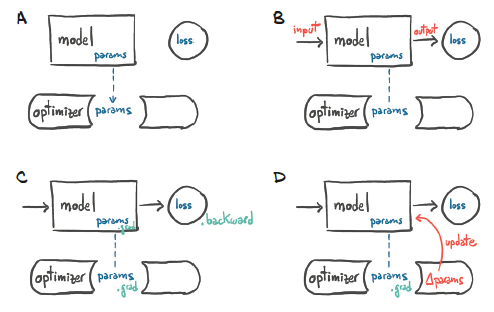
Every optimizer constructor in PyTorch takes a list of parameters (i.e., PyTorch tensors, typically with requires_grad set to True) as the first input. These parameters are retained within the optimizer object, allowing it to update their values and access their grad attribute.

This process is illustrated in Figure 6, which details the following steps:

1. A: Parameter Reference: The optimizer holds a reference to the parameters.
2. B: Loss Computation: After a loss is computed from the inputs.
3. C: Gradient Calculation: A call to .backward() populates the .grad attribute of the parameters.
4. D: Parameter Update: The optimizer accesses the .grad attributes and updates the parameter values accordingly.

Figure 6: Steps showing how the optimizer updates the values and gradients of the parameters. {#figure-6}

Forward and Backward Propagation

During typical machine learning model training, the model parameters are utilized in the forward pass and updated in the backward pass. The example below demonstrates how data, loss, and optimizer interact in this process.

# The optimizer holds a reference to the parameters. 
optimizer = torch.optim.SGD(model.parameters(), lr=0.01)

for epoch in range(num_epochs):
    for data, targets in dataloader:
        # Forward pass: compute model predictions and loss
        outputs = model(data)
        loss = loss_fn(outputs, targets)
        
        # Backward pass: compute gradients
        optimizer.zero_grad()  # Clear previous gradients
        loss.backward()  # Calculate new gradients
        
        # Update model parameters
        optimizer.step()  # Apply gradients to update parameters

In this example:

• Forward Pass: The model processes the input data to generate predictions (outputs), and the loss function (loss_fn) computes the loss based on these predictions and the actual targets.
• Backward Pass: Gradients are computed by calling loss.backward(), which populates the grad attributes of the model parameters.
• Parameter Update: The optimizer updates the model parameters using the computed gradients by calling optimizer.step().

Modules

The torch.nn.Module class is a base class in PyTorch for creating neural network models. It automatically tracks and manages parameters of the layers defined within the model. These parameters are registered as torch.nn.Parameter instances, which are Tensors with the additional property requires_grad=True. Modules can also contain other Modules, allowing for complex model architectures by nesting layers and sub-modules.

It is possible to directly use existing subclasses of nn.Module, such as nn.Linear, by defining:

model = nn.Linear(128, 10)

Alternatively, a customized subclass inheriting from nn.Module can be built, where the __init__() and forward() methods are defined. An example is found below.

import torch
import torch.nn as nn
import torch.nn.functional as F

class MyNetwork(nn.Module):
    def __init__(self):
        super(MyNetwork, self).__init__()
        self.fc1 = nn.Linear(128, 64)
        self.fc2 = nn.Linear(64, 10)

    def forward(self, x):
        x = F.relu(self.fc1(x))
        x = self.fc2(x)
        return x

model = MyNetwork()

SubModules

A module can have one or more submodules (subclasses of nn.Module) as attributes, and it will be able to track their parameters as well. This allows for the construction of more complex models by composing them from simpler submodules.

Here is an example of using a submodule:

class SubModule(nn.Module):
    def __init__(self):
        super(SubModule, self).__init__()
        self.fc = nn.Linear(128, 64)

    def forward(self, x):
        return F.relu(self.fc(x))

class MyNetwork(nn.Module):
    def __init__(self):
        super(MyNetwork, self).__init__()
        self.submodule = SubModule()
        self.fc = nn.Linear(64, 10)

    def forward(self, x):
        x = self.submodule(x)
        x = self.fc(x)
        return x

model = MyNetwork()

In the example above, the parameters of SubModule will be tracked automatically by MyNetwork.

However, submodules must be top-level attributes, not buried inside list or dict instances! Otherwise, the optimizer will not be able to locate the submodules (and, hence, their parameters). For situations where your model requires a list or dict of submodules, PyTorch provides nn.ModuleList and nn.ModuleDict.

An example of ModuleList is found below:

class MyModule(nn.Module):
    def __init__(self):
        super().__init__()
        self.linears = nn.ModuleList([nn.Linear(10, 10) for _ in range(10)])

    def forward(self, x):
        # ModuleList can act as an iterable or be indexed using ints
        for i, layer in enumerate(self.linears):
            x = self.linears[i // 2](x) + layer(x)
        return x

In this example, ModuleList is used to store a list of linear layers. This ensures that all submodules are properly registered and their parameters are tracked by the optimizer.

Forward Propagation

It’s important to note that the __call__() function in the nn.Module class includes the forward() function, but it also performs other crucial tasks before and after calling forward(). Therefore, when performing a forward pass, you should call model(X) instead of model.forward(X). Calling model.forward(X) directly can lead to silent errors.

Sequential Module

The torch.nn.Sequential class serves as a sequential container for stacking neural network modules in a linear order.

Modules are added to it in the order they are passed in the constructor. Alternatively, an OrderedDict of modules can be provided. The forward() method of Sequential accepts any input and passes it through the first module it contains. It then sequentially chains the outputs to inputs for each subsequent module, eventually returning the output of the last module.

One significant advantage of using Sequential is that it enables treating the entire container as a single module. Any transformation applied to the Sequential applies to each of the modules it stores, as each is registered as a submodule of the Sequential.

Here is an example of initializing a sequential module:

model = nn.Sequential(
    nn.Linear(1, 13),  # Linear layer with 1 input and 13 outputs
    nn.Tanh(),         # Hyperbolic tangent activation function
    nn.Linear(13, 1)   # Linear layer with 13 inputs and 1 output
)

Alternatively, the example of using OrderedDict can be found below, where more explanatory names are added for the submodules:

from collections import OrderedDict
model = nn.Sequential(
  OrderedDict([
    ('hidden_linear', nn.Linear(1, 8)),
    ('hidden_activation', nn.Tanh()),
    ('output_linear', nn.Linear(8, 1))
    ]
  )
)